BT Question P1-T2-20-16-1: Univariate regression: Inflation versus unemployment (using gt package to display table)
Background
BT is known for our tough training-style practice questions, but I wanted to take it further and add more realism. I’ve been writing a fresh question sets on the regression topics; I’m always writing new questions! It takes more time, but in these regression sets I’ve been pulling actual datasets. For this question, I pulled inflation and unemployment rates from the FRED database (see below). In combination with actual code-based applications, these new question sets are much more realistic than typical exam-prep fare. Let’s face it: in the real world, quantitative tasks (e.g., regression) are performed in software, not with calculators. In a way, it’s our responsibility to help candidates get exposure to tools that are actually useful. We’ve always been the only FRM exam prep provider (EPP) who develops virtually the entire, broad array of quantitative risk (FRM) topics in spreadsheet workbooks (this is a massive construction of hundreds of spreadsheets that has taken me the better part of a decade to build). Now I’ve started to develop associated code-based applications for the ultimate in realistic study material.
Using the gt package to render the regression output table
I thought I’d try the gt package to see if I could improve the presentation of the regression output table. It’s fairly intuitive but a little unexpected because you pipe (“%>%”) additional format features.
This question (my first in the new regression set) reads as follows:
“20.16.1. Debra is an analyst at a governmental agency. Her boss asked her to investigate whether the Phillips curve applies during high-inflation regimes. To answer the question, Debra collected data from the FRED database at the St. Louis Fed (https://fred.stlouisfed.org/). The Phillips curve describes an inverse relationship between unemployment rates and inflation rates; https://en.wikipedia.org/wiki/Phillips_curve. Debra collected monthly data and she regressed the inflation rate against the unemployment rate (conditional on high-inflation regimes). Her independent variable is unemployment rate (FRED code: UNRATE) and here dependent variable is the Inflation rate (CPIAUCSL). The units are percentages not decimals; e.g., the dataset includes the month of January in 1982 when the unemployment rate was 8.9 and the inflation rate was 6.38. Her regression results are presented below.”
We load the packages
library(tidyverse)
library(gt) # library(reactable) is another table package I haven't used
library(alfred) # Direct access to FRED
library(broom)
And then see if we might find a super-simple (ie, linear) Phillips curve (BT Question P1.T2.20.16.1)
startdate <- "1980-01-01"
enddate <- "2020-01-01"

# Phillips x = unemployment
unrate <- get_fred_series("UNRATE", "Unemployment", observation_start = startdate, observation_end = enddate)
inflation <- get_fred_series("CPIAUCSL", "inflation", observation_start = startdate, observation_end = enddate)
inflation_rate <- get_fred_series("PCETRIM12M159SFRBDAL", "Inflation_Rate", observation_start = startdate, observation_end = enddate)
df1 <- cbind(inflation, unrate, inflation_rate)
df1 <- df1[ , c(1,2, 4, 6)]
df2 <- df1 %>% filter(Inflation_Rate > 4.3)
df_fit <- lm(Inflation_Rate ~ Unemployment, data = df2)
summary(df_fit)
##
## Call:
## lm(formula = Inflation_Rate ~ Unemployment, data = df2)
##
## Residuals:
## Min 1Q Median 3Q Max
## -1.27252 -0.22807 -0.02961 0.25143 0.83596
##
## Coefficients:
## Estimate Std. Error t value Pr(>|t|)
## (Intercept) 16.38811 0.47300 34.65 <2e-16 ***
## Unemployment -1.10565 0.05572 -19.84 <2e-16 ***
## ---
## Signif. codes: 0 '***' 0.001 '**' 0.01 '*' 0.05 '.' 0.1 ' ' 1
##
## Residual standard error: 0.4726 on 38 degrees of freedom
## Multiple R-squared: 0.912, Adjusted R-squared: 0.9097
## F-statistic: 393.8 on 1 and 38 DF, p-value: < 2.2e-16df_fit_tidy <- tidy(df_fit)
gt_table <- gt(df_fit_tidy)
# This is the standard gt table which is an improvement
gt_table| term | estimate | std.error | statistic | p.value |
|---|---|---|---|---|
| (Intercept) | 16.38811 | 0.47300171 | 34.64705 | 2.328227e-30 |
| Unemployment | -1.10565 | 0.05571874 | -19.84342 | 1.186893e-21 |
# But here we'll utilize the pipe to specifically style the table
gt_table <-
  gt_table %>%
  tab_options(
    table.font.size = 14
  ) %>%
  tab_style(
    style = cell_text(weight = "bold"),
    locations = cells_body()
  ) %>%
  tab_header(
    title = "Inflation Rate (CPIAUCSL) regressed against Unemployment Rate (UNRATE)",
    subtitle = md("1980 to 2020 Monthly but conditioned on high inflation regimes")
  ) %>%
  tab_source_note(
    source_note = md("Source: FRED at https://fred.stlouisfed.org/")
  ) %>% cols_label(
    term = "Coefficient",
    estimate = "Estimate",
    std.error = "Std Error",
    statistic = "t-stat",
    p.value = "p value"
  ) %>% fmt_number(
    columns = vars(estimate, std.error, statistic),
    decimals = 3
  ) %>% fmt_scientific(
    columns = vars(p.value),
  ) %>%
  tab_options(
    heading.title.font.size = 14,
    heading.subtitle.font.size = 12
  ) %>%
  tab_footnote(
    footnote = "Filtered on months with inflation >4.3% deliberately to generate regression results",
    locations = cells_title("subtitle")
  )

gt_table| Inflation Rate (CPIAUCSL) regressed against Unemployment Rate (UNRATE) | ||||
|---|---|---|---|---|
| 1980 to 2020 Monthly but conditioned on high inflation regimes1 | ||||
| Coefficient | Estimate | Std Error | t-stat | p value |
| (Intercept) | 16.388 | 0.473 | 34.647 | 2.33 × 10⁻³⁰ |
| Unemployment | −1.106 | 0.056 | −19.843 | 1.19 × 10⁻²¹ |
| Source: FRED at https://fred.stlouisfed.org/ | ||||
|
1
Filtered on months with inflation >4.3% deliberately to generate regression results
|
||||
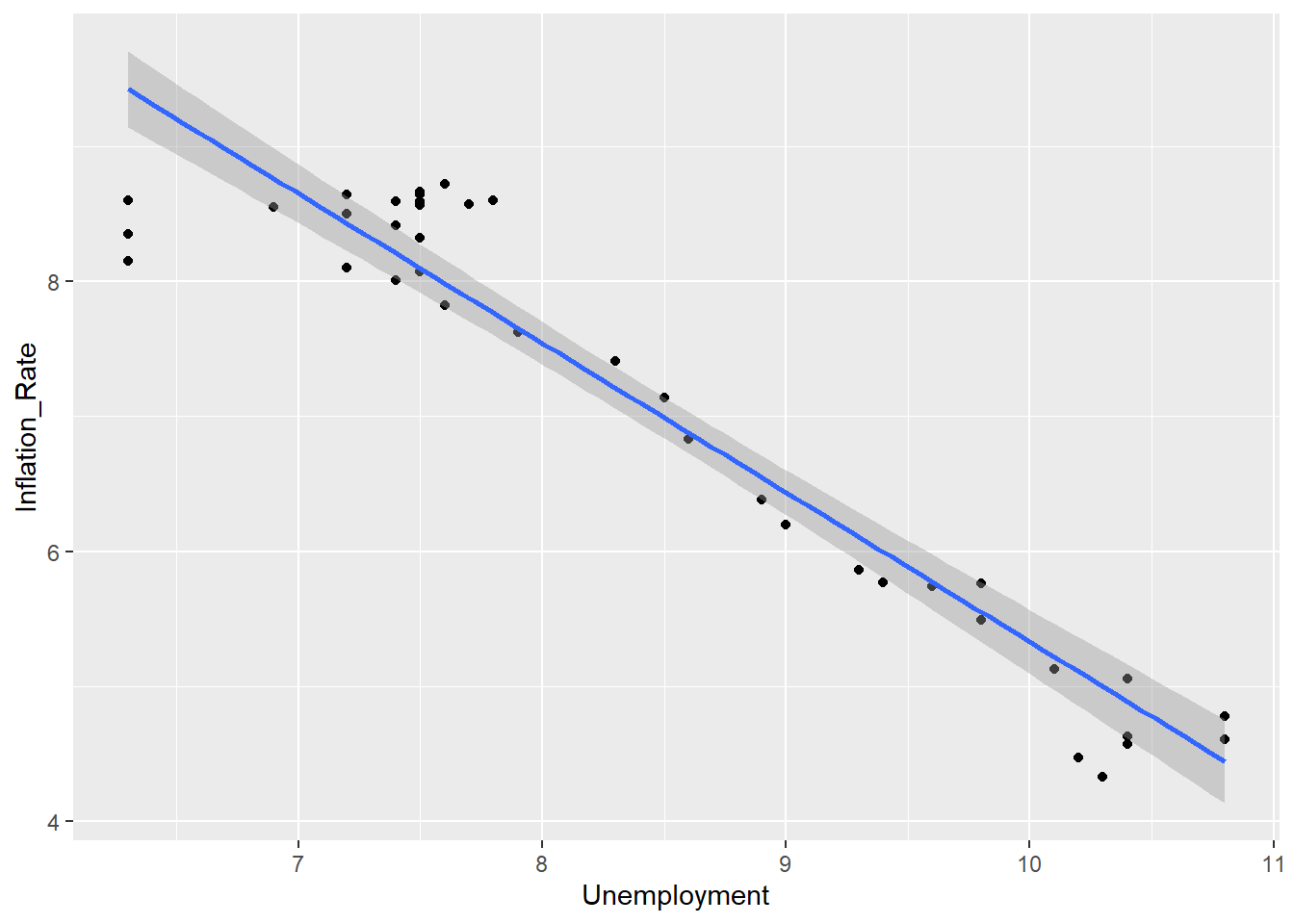
The question does not utilize a scatterplot but here it is anyway
df2 %>% ggplot(aes(Unemployment, Inflation_Rate)) +
  geom_point() +
  geom_smooth(method = "lm")
## `geom_smooth()` using formula 'y ~ x'