BT Question Set P1-T2-20-21-3: White Noise (WN) Process

P1-T2-20-21-3: White Noise (WN) Process)

20.21.3. Barbara was delighted to learn that she can easily simulate white noise in R with a single command. She learned that she can use arima.sim(model = list(order = c(0,0,0)), n = 100) to generate white noise with an ARIMA(0,0,0) model over a length of 100 days. She wants the shocks to have a Poisson distribution so she uses the command arima.sim(model = list(order = c(0,0,0)), n = 100, rand.gen = function(n, …) rpois(n, lambda = 10)) which assumes a Poisson distribution. Below is a plot of the white noise (top panel) and its associated autocorrelation function (ACF, bottom panel).

# Simulate a WN model with list(order = c(0, 0, 0))
# white_noise <- arima.sim(model = list(order = c(0,0,0)), n = 100)
# white_noise_1_tb  <- as_tibble(white_noise) %>% rowid_to_column()
# p1 <- ggplot(white_noise_1_tb, aes(x = rowid, y = x)) + geom_line()
# p2 <- ggAcf(white_noise)
# grid.arrange(p1, p2)

library(tidyverse)

## -- Attaching packages --------------------------------------------------------------------------------- tidyverse 1.3.0 --

## v ggplot2 3.3.2     v purrr   0.3.4
## v tibble  3.0.3     v dplyr   1.0.2
## v tidyr   1.1.2     v stringr 1.4.0
## v readr   1.3.1     v forcats 0.5.0

## -- Conflicts ------------------------------------------------------------------------------------ tidyverse_conflicts() --
## x dplyr::filter() masks stats::filter()
## x dplyr::lag()    masks stats::lag()

library(forecast)

## Registered S3 method overwritten by 'quantmod':
##   method            from
##   as.zoo.data.frame zoo

library(patchwork)
library(extrafont)

## Registering fonts with R

library(ggthemes)
# library(ggfortify)
# library(cowplot)

set.seed(58)

# Simulate a WN model with list(order = c(0, 0, 0))
# dat_wn <- arima.sim(model = list(order = c(0,0,0)), n = 100)
dat_wn <- arima.sim(model = list(order = c(0,0,0)), n = 100, 
                         rand.gen = function(n, ...) rpois(n, lambda = 10))
dat_wn_tbl <- bind_cols(dat_wn) %>% rowid_to_column() %>% rename(value_y = ...1 )

## New names:
## * NA -> ...1

process_color = "#266935"
p1 <- dat_wn_tbl %>% ggplot(aes(x = rowid, y = value_y)) +
  geom_line(size= 1, color = process_color) +
  ylab("Y Value") +
  xlab("Process (100 days)") + 
  theme_bw() + 
  theme(
    text = element_text(family = "Calibri"),
    plot.title = element_blank(),
    axis.title.x = element_text(size = 14, face = "bold"),
    axis.title.y = element_text(size = 14, face = "bold", color = process_color),
    axis.text.x = element_text(size = 14, face = "bold"),
    axis.text.y = element_text(size = 14, face= "bold"),
    panel.background = element_blank(),
    panel.grid.major.x = element_blank(),
    panel.grid.major.y = element_line(color="grey"),
    panel.border = element_blank()
  )

#p2 <- ggAcf(dat_wn)

p2 <- ggAcf(dat_wn) + 
  xlab("Lags") + 
  theme_bw() +
  geom_segment(size = 3) +
  theme(
    text = element_text(family = "Calibri"),
    plot.title = element_blank(),
    axis.title.x = element_text(size = 14, face = "bold"),
    axis.title.y = element_text(size = 14, face = "bold"),
    axis.text.x = element_text(size = 14, face = "bold"),
    axis.text.y = element_text(size = 14, face= "bold"),
    panel.background = element_blank(),
    panel.grid.major.x = element_blank(),
    panel.grid.major.y = element_line(color="grey"),
    panel.border = element_blank()
  )


# grid.arrange(p1, p2)

p1/p2

## Don't know how to automatically pick scale for object of type ts. Defaulting to continuous.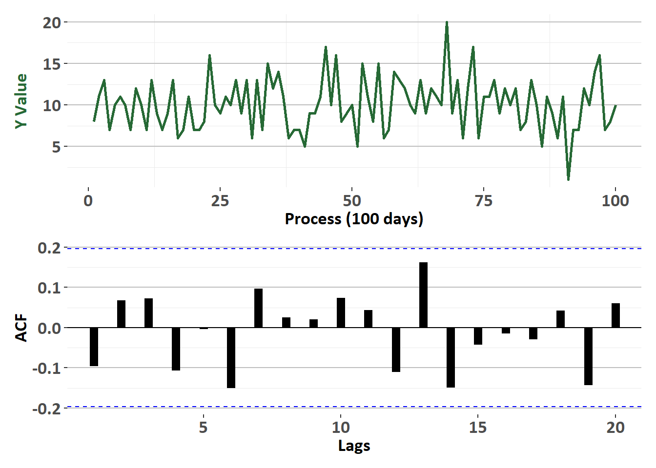

s5 <- arima.sim(model = list(order = c(0,0,0)), n = 100, 
                         rand.gen = function(n, ...) rpois(n, lambda = 10))

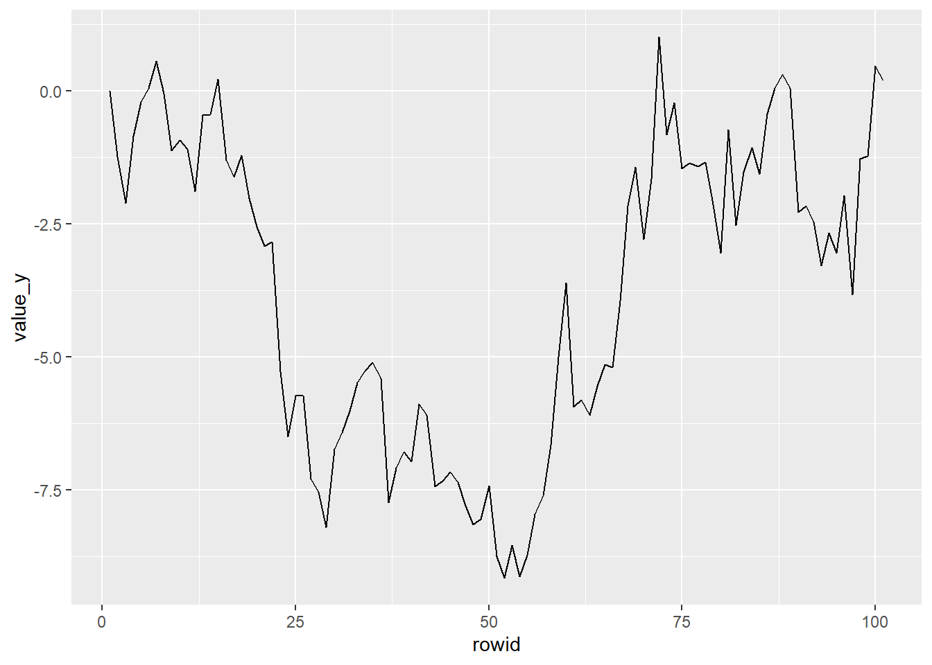
dat_rw <- arima.sim(model = list(order = c(0,1,0)), n = 100)
dat_rw_tbl <- bind_cols(dat_rw) %>% rowid_to_column() %>% rename(value_y = ...1 )

## New names:
## * NA -> ...1

dat_rw_tbl %>% ggplot(aes(x = rowid, y = value_y)) + geom_line()

## Don't know how to automatically pick scale for object of type ts. Defaulting to continuous.