BT Question Set P1-T2-20-24-2: Box-Pierce
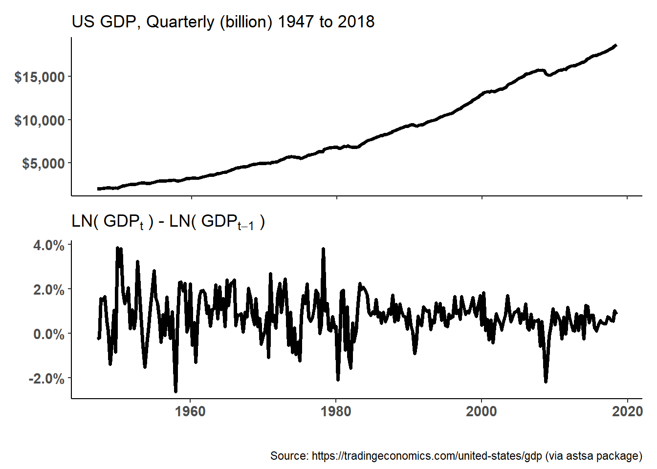
20.24.2. Elizabeth is an economist tasked with modeling quarterly gross domestic product (GDP) in the United States. She starts with the plots displayed below. The raw data is displayed in the upper; she observes this GDP trend is obviously not stationary (why?). She then performs a typical transformation on the raw data: she takes the difference of the natural log of the quarterly GPD values. This plot is displayed in the lower panel. Because LN[GDP(t)] - LN(GDP(t-1)] = LN[GDP(t)/GDP(t-1)], this lower panel plots continuously compounded returns (aka, monthly log returns). First differencing the log returns occasionally renders the non-stationary trend into a stationary process.
library(tidyverse)## -- Attaching packages --------------------------------------------------------------------------------- tidyverse 1.3.0 --## v ggplot2 3.3.2 v purrr 0.3.4
## v tibble 3.0.3 v dplyr 1.0.2
## v tidyr 1.1.2 v stringr 1.4.0
## v readr 1.3.1 v forcats 0.5.0## -- Conflicts ------------------------------------------------------------------------------------ tidyverse_conflicts() --
## x dplyr::filter() masks stats::filter()
## x dplyr::lag() masks stats::lag()library(scales)##
## Attaching package: 'scales'## The following object is masked from 'package:purrr':
##
## discard## The following object is masked from 'package:readr':
##
## col_factorlibrary(forecast)## Registered S3 method overwritten by 'quantmod':
## method from
## as.zoo.data.frame zoolibrary(tseries)
library(ggthemes)
library(ggfortify)## Registered S3 methods overwritten by 'ggfortify':
## method from
## autoplot.Arima forecast
## autoplot.acf forecast
## autoplot.ar forecast
## autoplot.bats forecast
## autoplot.decomposed.ts forecast
## autoplot.ets forecast
## autoplot.forecast forecast
## autoplot.stl forecast
## autoplot.ts forecast
## fitted.ar forecast
## fortify.ts forecast
## residuals.ar forecastlibrary(fpp2)## -- Attaching packages ---------------------------------------------------------------------------------------- fpp2 2.4 --## v fma 2.4 v expsmooth 2.3## -- Conflicts ------------------------------------------------------------------------------------------- fpp2_conflicts --
## x scales::discard() masks purrr::discard()library(gt)
library(astsa)##
## Attaching package: 'astsa'## The following objects are masked from 'package:fma':
##
## chicken, sales## The following object is masked from 'package:fpp2':
##
## oil## The following object is masked from 'package:forecast':
##
## gaslibrary(patchwork)
# library(gridExtra)
gdp_log <- diff(log(gdp))
# ts.plot(gdp)
# ts.plot(gdp_log)
p1_gdp <- autoplot(gdp, size = 1.3) + labs(
title = "US GDP, Quarterly (billion) 1947 to 2018"
) + theme_classic() + theme(
axis.title.x = element_blank(),
axis.title.y = element_blank(),
axis.text.x = element_blank(),
axis.text.y = element_text(size = 11, face = "bold")
) + scale_y_continuous(labels = dollar_format())## Scale for 'y' is already present. Adding another scale for 'y', which will
## replace the existing scale.p2_gdp_log <- autoplot(gdp_log, size = 1.3) + labs(
title = bquote("LN("~GDP[t]~ ") - LN("~GDP[t-1]~")")
) + theme_classic() + theme(
axis.title.y = element_blank(),
axis.text.x = element_text(size = 11, face = "bold"),
axis.text.y = element_text(size = 11, face = "bold")
) + scale_y_continuous(labels = label_percent(accuracy = .1))## Scale for 'y' is already present. Adding another scale for 'y', which will
## replace the existing scale.patchwork <- p1_gdp / p2_gdp_log
patchwork + plot_annotation(
caption = "Source: https://tradingeconomics.com/united-states/gdp (via astsa package)"
)
(on to the Box-Pierce…)
She then fits an autoregressive, AR(1), and moving average, MA(1), model to the log return series. This gives her three models: the log return series (called “diff_logs”), an AR(1) model, and an MA(1) model. She conducts a Box-Pierce test on each of these models; the test of the AR(1) and MA(1) is a test of the residuals. She selects two lags for the test, h = 10 and h = 20. The results of her Box-Pierce test are displayed below.
… Box-Pierce gt table (below) here …
If we assume her desired confidence level is 95.0%, which of the following statements is a TRUE statement with respect to an interpretation of her Box-Pierce test of the three models?
- None of the residuals are white noise; i.e., neither the transformed log returns nor AR(1) nor MA(1) is a candidate model
- The AR(1) is a candidate because its residuals appear to be approximately white noise
- The MA(a) is a candidate because its residuals appear to be approximately white noise
- All of the residuals are white noise; i.e., all three models are candidates
# install.packages("kableExtra")
# install.packages("gapminder")

ar1_gdp_log <- sarima(gdp_log, p = 1, d = 0, q = 0)
## initial value -4.673186
## iter 2 value -4.742918
## iter 3 value -4.742921
## iter 4 value -4.742923
## iter 5 value -4.742925
## iter 6 value -4.742925
## iter 6 value -4.742925
## final value -4.742925
## converged
## initial value -4.742229
## iter 2 value -4.742234
## iter 3 value -4.742245
## iter 3 value -4.742245
## iter 3 value -4.742245
## final value -4.742245
## converged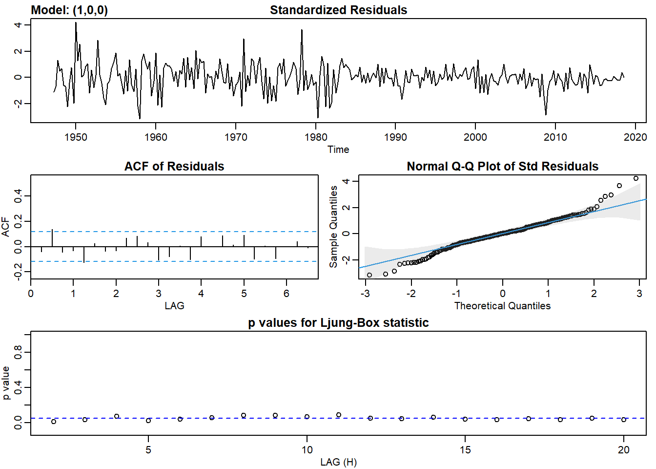
ma1_gdp_log <- sarima(gdp_log, p = 0, d = 0, q = 1)## initial value -4.672758
## iter 2 value -4.716609
## iter 3 value -4.723220
## iter 4 value -4.723481
## iter 5 value -4.723483
## iter 5 value -4.723483
## iter 5 value -4.723483
## final value -4.723483
## converged
## initial value -4.723444
## iter 1 value -4.723444
## final value -4.723444
## converged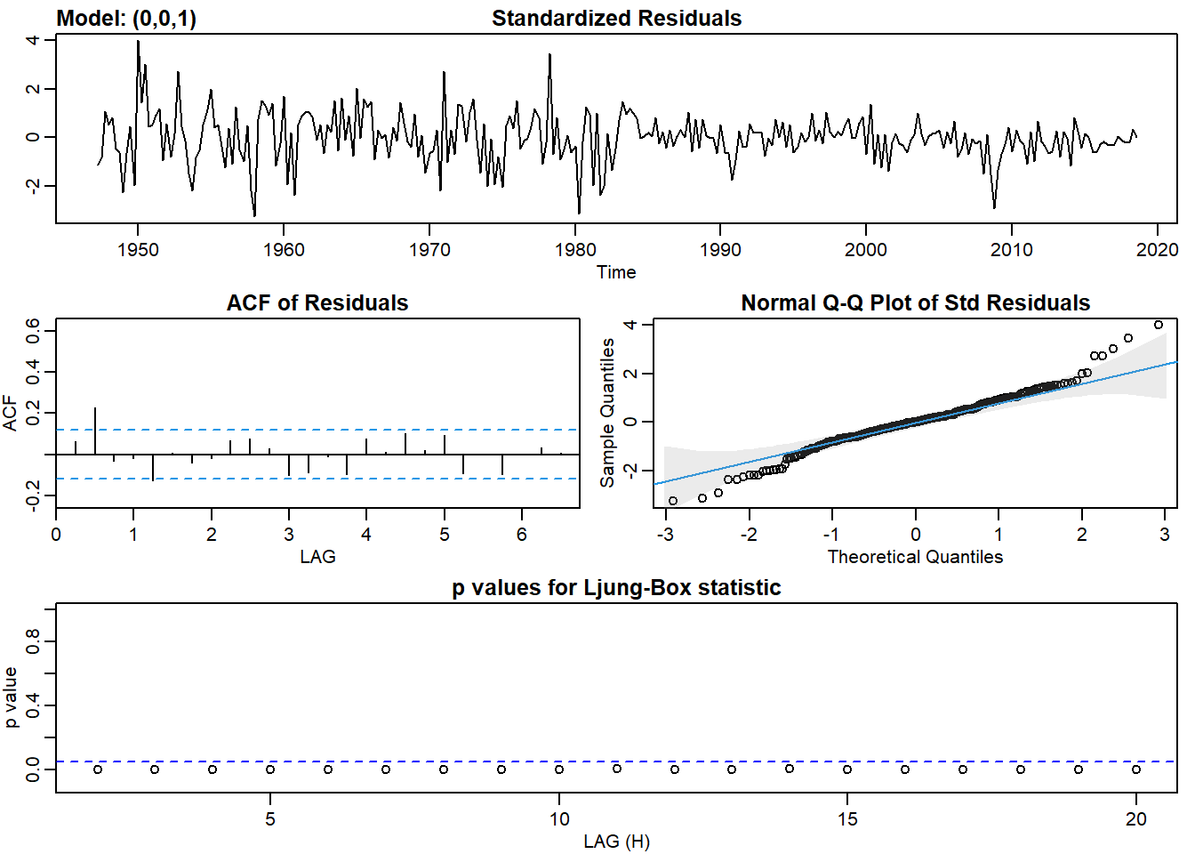
ma2_gdp_log <- sarima(gdp_log, p = 0, d = 0, q = 2)## initial value -4.672758
## iter 2 value -4.749239
## iter 3 value -4.750696
## iter 4 value -4.750723
## iter 5 value -4.750724
## iter 6 value -4.750725
## iter 7 value -4.750725
## iter 7 value -4.750725
## iter 7 value -4.750725
## final value -4.750725
## converged
## initial value -4.751078
## iter 2 value -4.751080
## iter 3 value -4.751080
## iter 4 value -4.751081
## iter 5 value -4.751081
## iter 5 value -4.751081
## iter 5 value -4.751081
## final value -4.751081
## converged
h_values <- c(10, 20)

# diff of logs
model = "diff_logs"
results_log_list <- h_values %>% map(~Box.test(gdp_log, lag = .))
log_statistic <- results_log_list %>% map_dbl("statistic")
log_p.value <- results_log_list %>% map_dbl("p.value")
log_cols <- data.frame(cbind(h_values, log_statistic, log_p.value))
log_all <- cbind(model, log_cols)
log_all <- log_all %>% rename(
  'h (lags)' = h_values,
  statistic = log_statistic,
  'p-value' = log_p.value
)

# AR(1)
model = "AR(1)"
results_ar1_list <- h_values %>% map(~Box.test(ar1_gdp_log$fit$residuals, lag = .))
ar1_statistic <- results_ar1_list %>% map_dbl("statistic")
ar1_p.value <- results_ar1_list %>% map_dbl("p.value")
ar1_cols <- data.frame(cbind(h_values, ar1_statistic, ar1_p.value))
ar1_all <- cbind(model, ar1_cols)
ar1_all <- ar1_all %>% rename(
  'h (lags)' = h_values,
  statistic = ar1_statistic,
  'p-value' = ar1_p.value
)

# MA(1)
model = "MA(1)"
results_ma1_list <- h_values %>% map(~Box.test(ma1_gdp_log$fit$residuals, lag = .))
ma1_statistic <- results_ma1_list %>% map_dbl("statistic")
ma1_p.value <- results_ma1_list %>% map_dbl("p.value")
ma1_cols <- data.frame(cbind(h_values, ma1_statistic, ma1_p.value))
ma1_all <- cbind(model, ma1_cols)
ma1_all <- ma1_all %>% rename(
  'h (lags)' = h_values,
  statistic = ma1_statistic,
  'p-value' = ma1_p.value
)

models_all <- rbind(log_all, ar1_all, ma1_all)
models_gt <- gt(models_all)

models_gt <-
  models_gt %>%
  tab_options(
    table.font.size = 14
  ) %>% tab_style(
    style = cell_text(weight = "bold"),
    locations = cells_body()
  ) %>% tab_style(
    style = cell_text(color = "cadetblue"),
    locations = cells_column_labels(
      columns = vars(model, 'h (lags)', statistic, 'p-value')
    )
  ) %>% tab_header(
    title = md("**Box-Pierce test statistics and p-values**"),
    subtitle = "AR(1) and MA(1) at lags of h = 10 and 20"
  ) %>% fmt_number(
    columns = vars(statistic, 'p-value'),
    decimals = 4
  ) %>% tab_source_note(
    source_note = md("Note: diff_logs = LN[GDP(t)] - LN[GPD(t-1)]")
  ) %>% tab_source_note(
    source_note = md("AR(1) and MA(1) are tests of residuals")
  ) %>% cols_width(
    vars(model, 'h (lags)') ~ px(80),
    vars(statistic, 'p-value') ~ px(90)
  ) %>% cols_label (
    model = md("**model**"),
    'h (lags)' = md("**h (lags)**"),
    statistic = md("**test stat**"),
    'p-value' = md("**p-value**")
  ) %>% cols_align(
    align = "center",
    columns = vars('h (lags)')
  ) %>% tab_options(
    heading.title.font.size = 16,
    heading.subtitle.font.size = 14
  )

models_gt| Box-Pierce test statistics and p-values | |||
|---|---|---|---|
| AR(1) and MA(1) at lags of h = 10 and 20 | |||
| model | h (lags) | test stat | p-value |
| diff_logs | 10 | 62.6228 | 0.0000 |
| diff_logs | 20 | 80.1439 | 0.0000 |
| AR(1) | 10 | 15.5465 | 0.1134 |
| AR(1) | 20 | 30.3091 | 0.0650 |
| MA(1) | 10 | 24.3689 | 0.0067 |
| MA(1) | 20 | 39.6618 | 0.0055 |
| Note: diff_logs = LN[GDP(t)] - LN[GPD(t-1)] | |||
| AR(1) and MA(1) are tests of residuals | |||