BT Question Set P1-T2-21-1: Non-stationary time series
21.1.1 This is a seasonal model without a trend
21.1.1 The following seasonal dummy model estimates the quarterly growth rate (in percentage terms) of housing starts … The model’s intercept (δ) equals +1.20 and the gamma coefficients are the following: γ(1) = -2.60, γ(2) = +7.90, and γ(3) = +1.80. According to this model, when does the growth rate peak?
# similar to GARP's EOC 11.8, there is no trend, only seasonality

c_delta <- 1.20; gamma <- c(-2.6, 7.9, 1.80, 0)
quarters <- rep(1:4, 5)
y = c_delta + gamma[quarters]
ts.plot(y)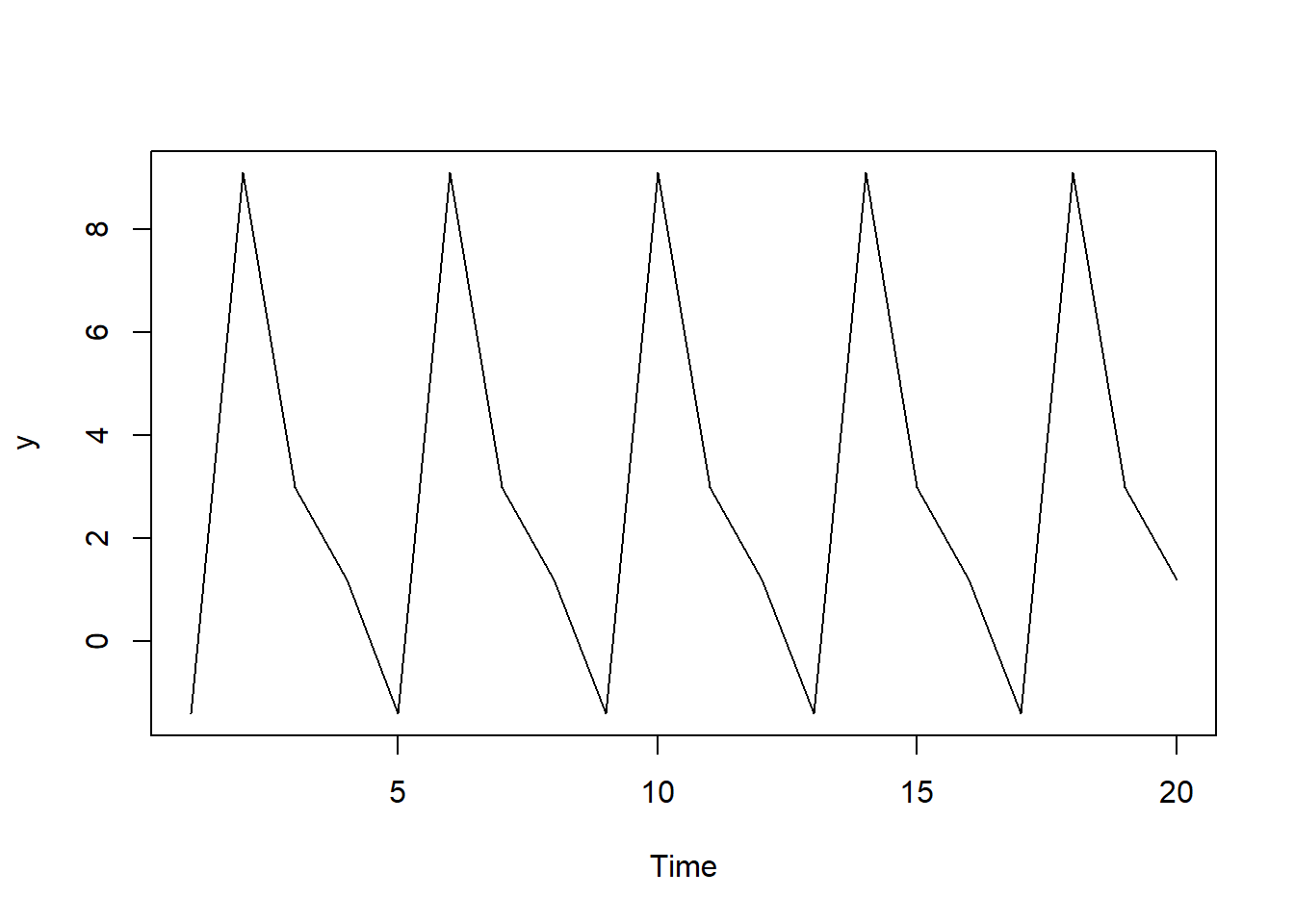
21.1.2 An AR(2) that is stationary as demonstrated by |roots| > 1.0 but also our ability to simulate
21.1.2. Peter wants to model the following AR(2) time series: Y(t) = 0.750Y(t-1) - 0.1250T(t-2) + e(t). He wonders if this AR(2) is stationary. He realizes that he can write this as a log polynomial …
# install.packages("polynom", repos = "http://cran.us.r-project.org")
library(polynom)

peters_poly <- polynomial(coef = c(1, -0.75, 0.125))
peters_poly
## 1 - 0.75*x + 0.125*x^2solve(peters_poly) # the roots (aka, zeros) are 2 and 4## [1] 2 4ar_2 <- arima.sim(model=list(order=c(2,0,0),ar = c(-0.75, 0.125)),n = 100)
ts.plot(ar_2)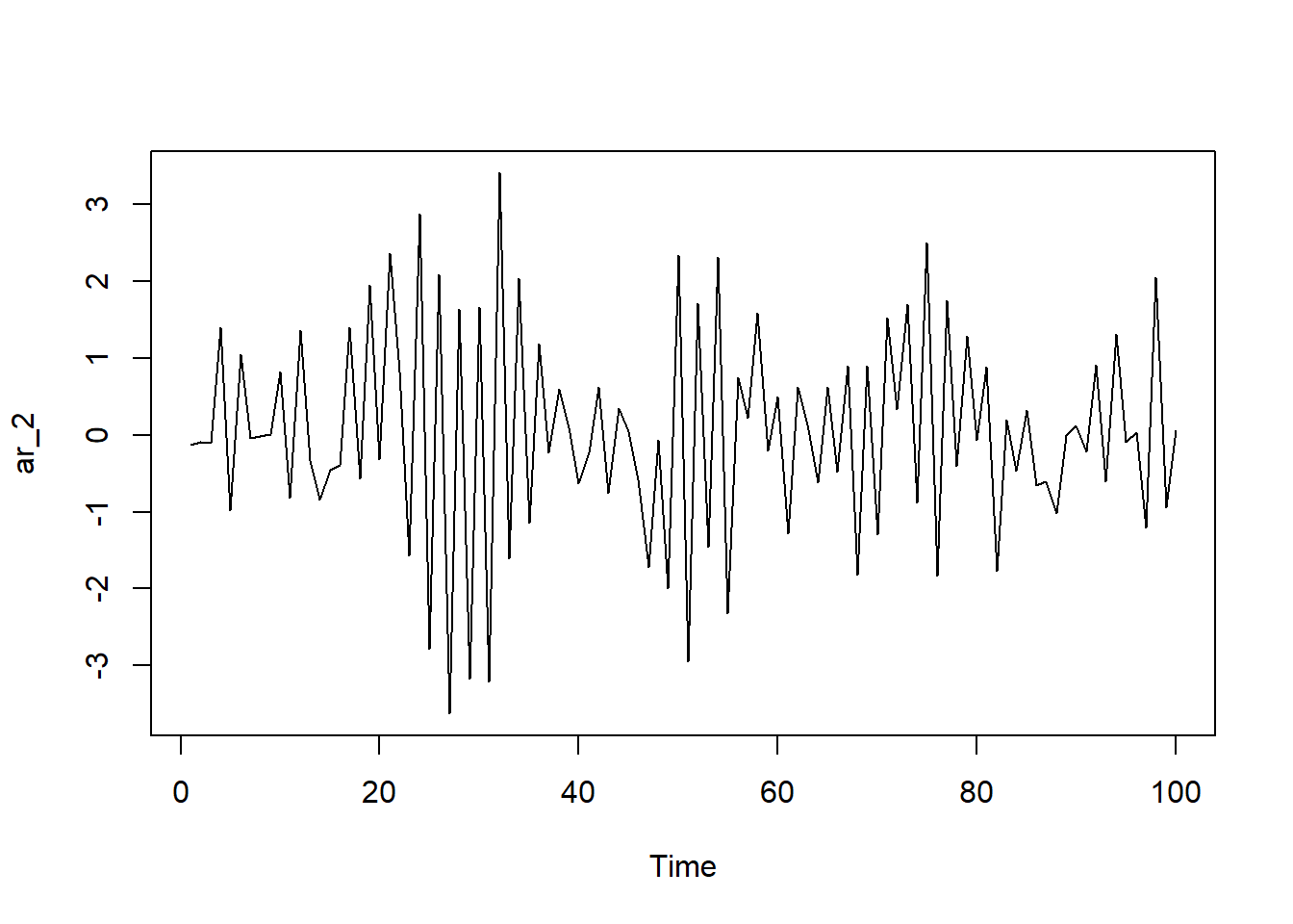
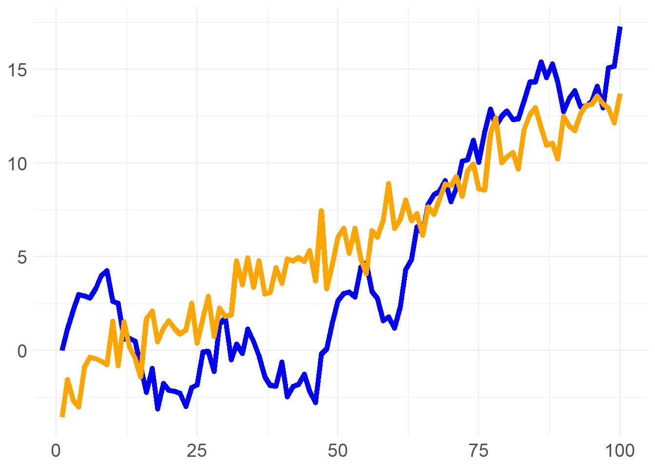
21.1.3 Compares a deterministic trend to a stochastic (random walk with drift) trend
21.1.3. Sally considers two series for her model: a linear trend model (aka, deterministic trend), and a random walk with drift. Each is simulated below (n = 100 steps)
library(tidyverse)## -- Attaching packages --------------------------------------------------------------------------------- tidyverse 1.3.0 --## v ggplot2 3.3.2 v purrr 0.3.4
## v tibble 3.0.3 v dplyr 1.0.2
## v tidyr 1.1.2 v stringr 1.4.0
## v readr 1.3.1 v forcats 0.5.0## -- Conflicts ------------------------------------------------------------------------------------ tidyverse_conflicts() --
## x dplyr::filter() masks stats::filter()
## x dplyr::lag() masks stats::lag()library(ggthemes)
library(RColorBrewer)
set.seed(28)
n <- 100
x <- 1:n
# white noise
white_noise <- arima.sim(model = list(order = c(0,0,0)), n = 100)
#linear trend
linear_tr <- -1.8 + 0.15*x
time_trend <- linear_tr + white_noise
rw_drift <- arima.sim(model = list(order = c(0,1,0)), n = n-1, mean = 0.4)
trends <- data.frame(
x,
time_trend,
rw_drift
)
p1 <- trends %>% ggplot(aes(x=x)) +
geom_line(aes(y=rw_drift), color = "blue", size = 2) +
geom_line(aes(y=time_trend), color = "orange", size = 2) +
theme_minimal() +
theme(
axis.title = element_blank(),
axis.text = element_text(size = 14)
)
p1## Don't know how to automatically pick scale for object of type ts. Defaulting to continuous.