BT Question P1-T2-20-16-2: Univariate regression: Portfolio versus benchmark returns

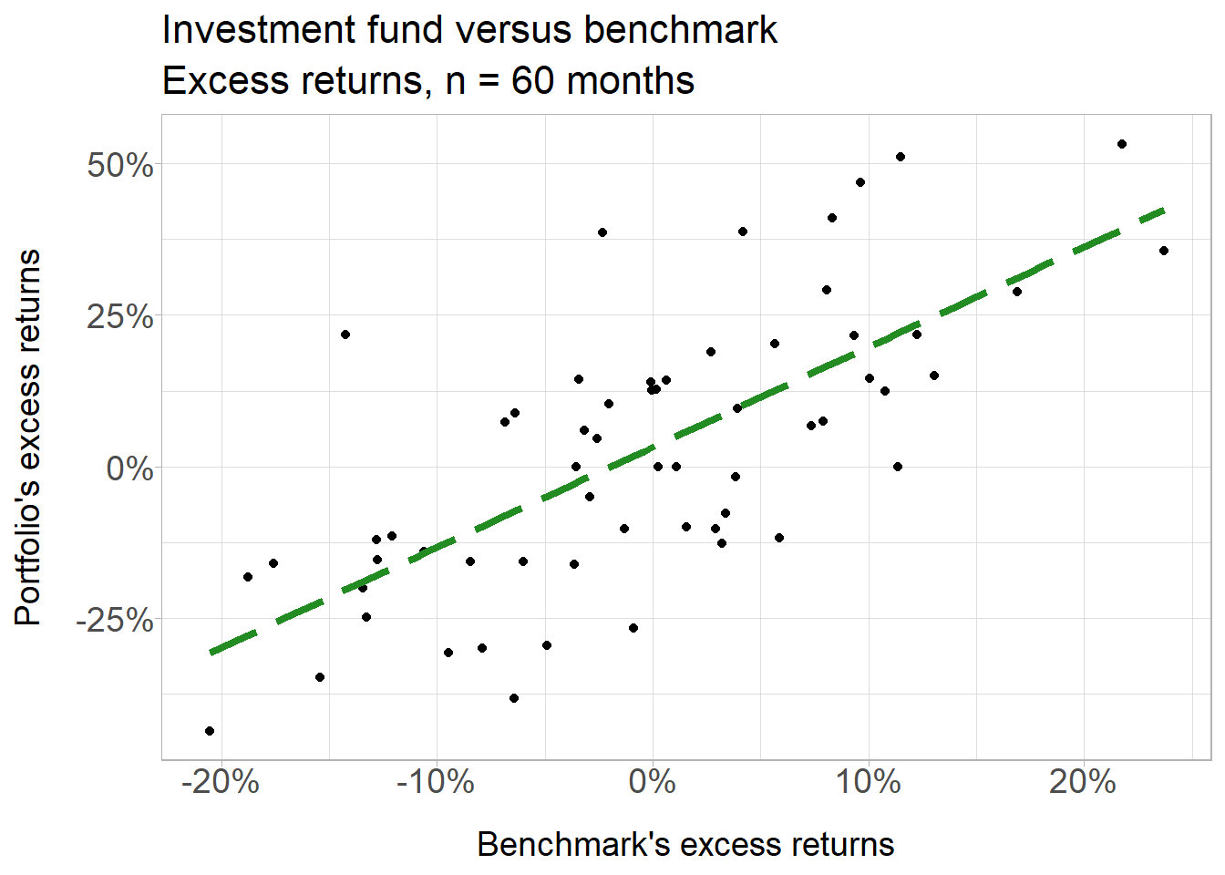
20.16.2. Peter is an analyst who is evaluating an investment fund whose managers claim has outperformed their benchmark. He collected monthly returns for the last five years; i.e., the sample size is excess return pairs over n = 60 months. He plots excess returns, which are defined as the returns in excess of the riskfree rate; ie., an excess return equals the gross return minus the riskfree rate. The scatterplot is displayed below:

scatterplot

The correlation coefficient is 0.708. In regard to the univariate data, the standard deviation of the portfolio’s returns is 22.84% and the standard deviation of the benchmark’s returns is 9.79%. The average excess return of the benchmark was -0.37% and the average excess return of the portfolio was 2.61%. Each of the following statements is true EXCEPT which is false?

library(tidyverse)
library(scales)
library(ggthemes)
# library(lmtest)

x_mu <- .01; x_sig <- .1

y_mu <- .03; y_sig <- .2

rho <-  0.72
months <- 60

#set.seed(59)
set.seed(158)

# 60  rows of random standard normals
returns <- tibble(index = 1:months)
returns$x1 <- rnorm(months) 
returns$y1 <- rnorm(months)

# make y2 correlated with y1; adjust location/scale
returns1 <- returns %>% mutate(
  y2 = rho*x1 + sqrt(1 - rho^2)*y1,
  r_x = x_mu + x1 * x_sig,
  r_y = y_mu + y2 * y_sig
)

x_sd <- sd(returns1$r_x)
y_sd <- sd(returns1$r_y)
rho_xy <- cor(returns1$r_x, returns1$r_y)
beta_yx <- rho_xy * y_sd / x_sd
x_mu_act <- mean(returns1$r_x)
y_mu_act <- mean(returns1$r_y)

sprintf("sample rho is %.4f. The standard deviation of Portfolio returns is ", rho_xy)

## [1] "sample rho is 0.7078. The standard deviation of Portfolio returns is "

paste("Portfolio standard deviation is", percent(y_sd, accuracy = .01))

## [1] "Portfolio standard deviation is 22.84%"

paste("Benchmark standard deviation is", percent(x_sd, accuracy = .01))

## [1] "Benchmark standard deviation is 9.79%"

paste("Portfolio average excess return is", percent(y_mu_act, accuracy = .01))

## [1] "Portfolio average excess return is 2.61%"

paste("Benchmark average excess return is", percent(x_mu_act, accuracy = .01))

## [1] "Benchmark average excess return is -0.37%"

sprintf("Beta(P,B) is %.3f", beta_yx) 

## [1] "Beta(P,B) is 1.652"

returns1_lm <- lm(r_y ~ r_x, data = returns1)
summary(returns1_lm)

## 
## Call:
## lm(formula = r_y ~ r_x, data = returns1)
## 
## Residuals:
##      Min       1Q   Median       3Q      Max 
## -0.30810 -0.11231 -0.01385  0.09922  0.42134 
## 
## Coefficients:
##             Estimate Std. Error t value Pr(>|t|)    
## (Intercept)  0.03231    0.02102   1.537     0.13    
## r_x          1.65219    0.21649   7.632 2.54e-10 ***
## ---
## Signif. codes:  0 '***' 0.001 '**' 0.01 '*' 0.05 '.' 0.1 ' ' 1
## 
## Residual standard error: 0.1627 on 58 degrees of freedom
## Multiple R-squared:  0.501,  Adjusted R-squared:  0.4924 
## F-statistic: 58.24 on 1 and 58 DF,  p-value: 2.543e-10

returns1 %>% ggplot(aes(x = r_x, y = r_y)) +
  geom_point() +
  geom_smooth(method = "lm", se = FALSE, color = "forestgreen", linetype = "longdash", size = 1.5) +
  labs(title = "Investment fund versus benchmark", 
       subtitle = "Excess returns, n = 60 months") +
  xlab("Benchmark's excess returns") +
  ylab("Portfolio's excess returns") +
  scale_x_continuous(labels = percent_format(accuracy = 1)) +
  scale_y_continuous(labels = percent_format(accuracy = 1)) +
  theme_light() +
  theme(
    plot.title = element_text(size = 16),
    plot.subtitle = element_text(size = 16),
    axis.title.y = element_text(size = 14),
    axis.title.x = element_text(size = 14),
    axis.text.x = element_text(size = 14, margin = margin(b = 10)),
    axis.text.y = element_text(size = 14, margin = margin(l = 10))
  )

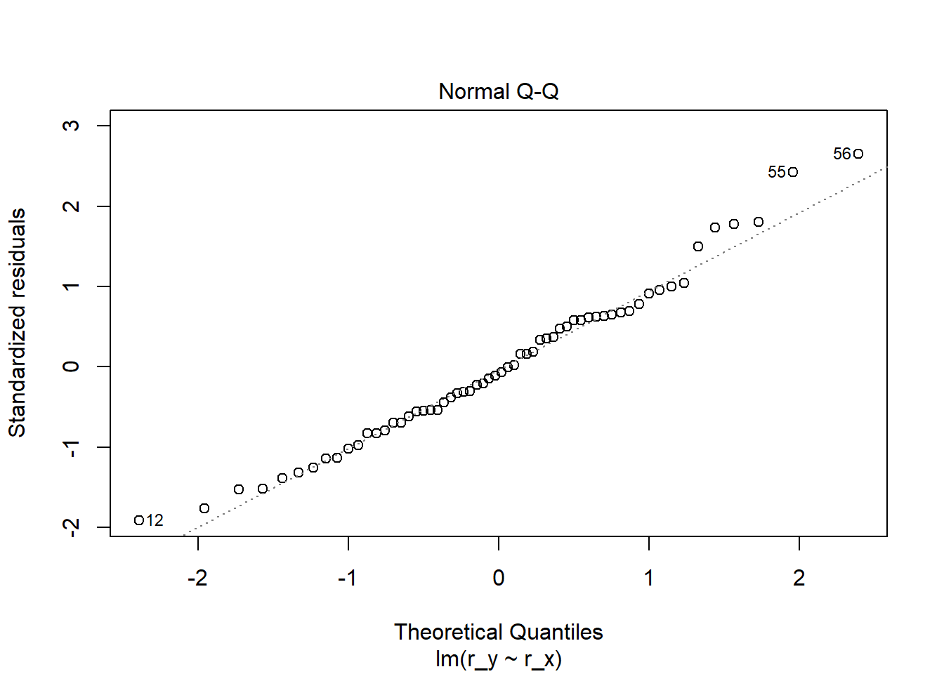
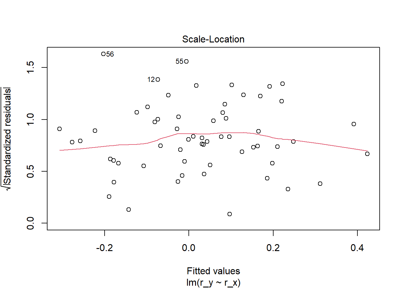
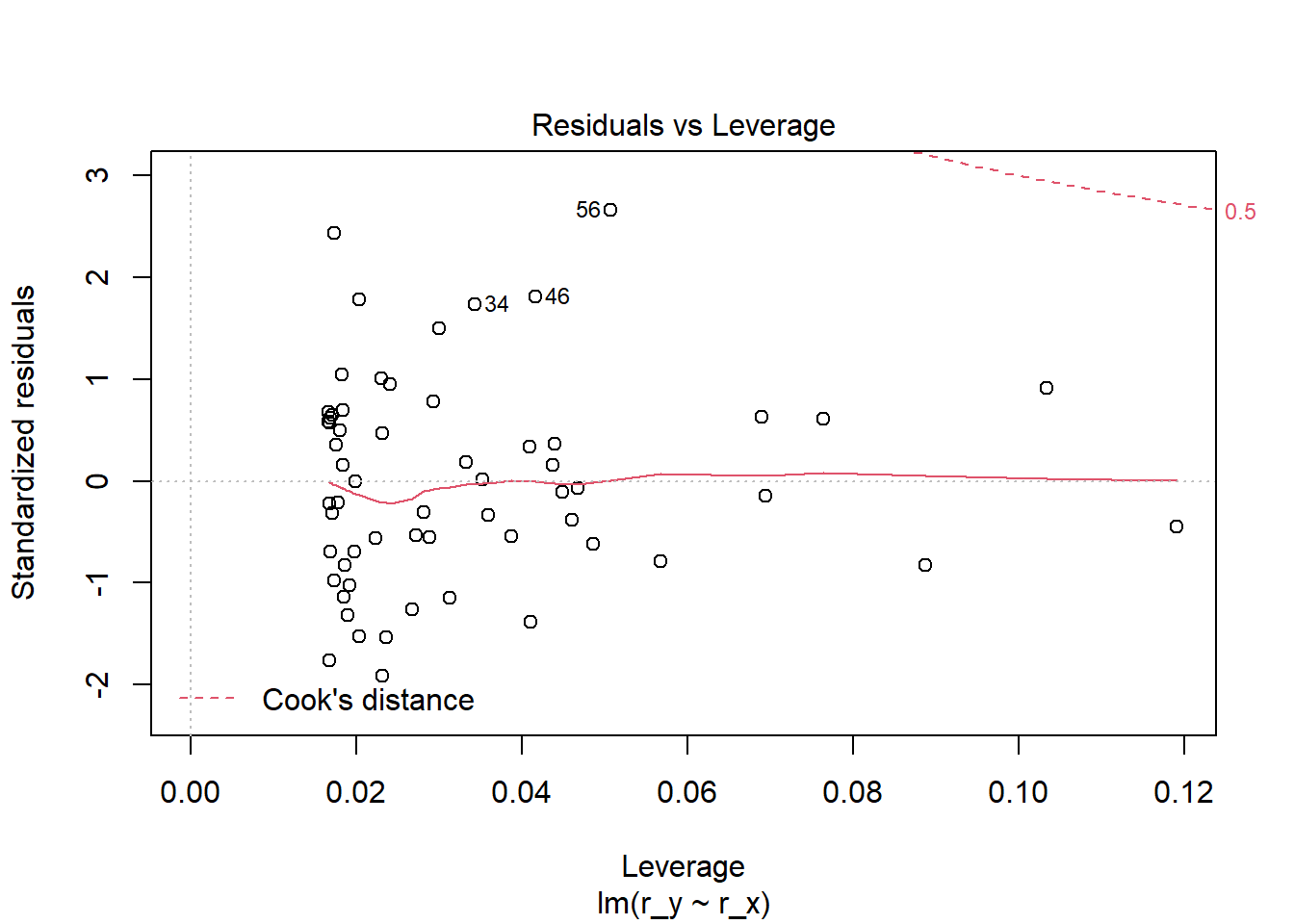
plot(returns1_lm)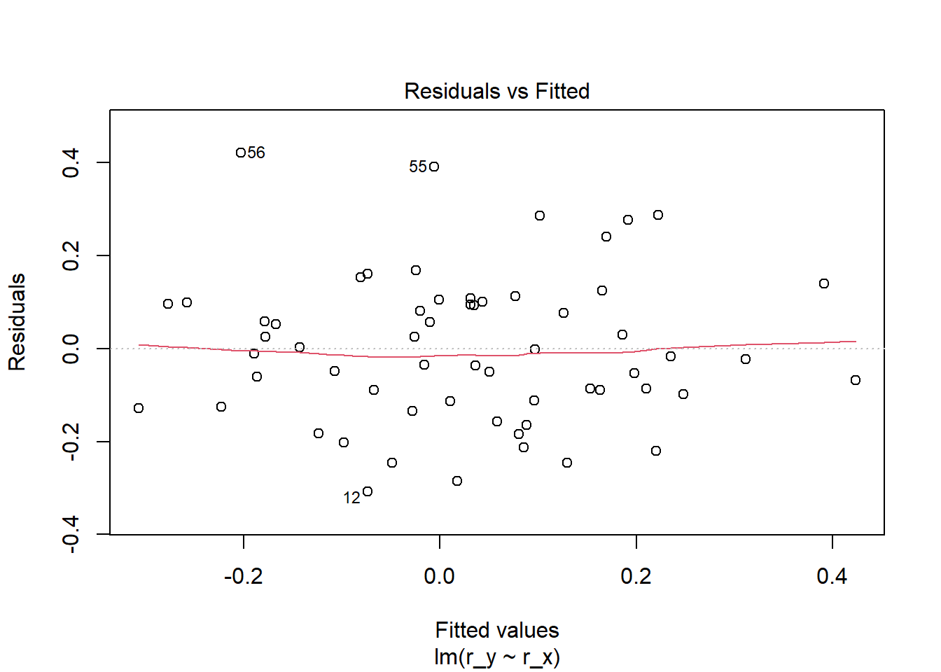

new.df <- data.frame(r_x = c(x_mu_act, 0, seq(from = 0.01, to = 0.1, by = .01)))
new.df$predicted_y <- predict(returns1_lm, new.df)
new.df

##             r_x predicted_y
## 1  -0.003740684  0.02613168
## 2   0.000000000  0.03231199
## 3   0.010000000  0.04883388
## 4   0.020000000  0.06535577
## 5   0.030000000  0.08187766
## 6   0.040000000  0.09839955
## 7   0.050000000  0.11492143
## 8   0.060000000  0.13144332
## 9   0.070000000  0.14796521
## 10  0.080000000  0.16448710
## 11  0.090000000  0.18100899
## 12  0.100000000  0.19753088

intercept_predict <- (0 - x_mu_act)*beta_yx + y_mu_act
intercept_predict_round <- (0 - round(x_mu_act,4))*beta_yx + round(y_mu_act,4)
intercept_predict

## [1] 0.03231199

intercept_predict_round

## [1] 0.0322131